Dimensions of Return
By Ehren Stanhope
April 2018
There are three universal dimensions of return that drive the performance of all strategies—regardless of investment style or asset class: consistency, magnitude, and conviction. These dimensions serve as levers that can increase or decrease performance of any strategy. They also provide context for why portfolios are constructed in the manner that they are. This piece will attempt to create a framework for evaluation and to identify which of the dimensions have a disproportionate influence on performance. In applying the framework to the Russell 1000® and 2000® Value, and the top and bottom large and small cap managers, I find that the dimensions provide insight as to which skills differentiate top and bottom professional managers.
Investing in any asset class, be it public equities or seed stage venture capital consists of two critical decisions: what to buy and sell (selection) and in what proportions (weighting). To understand the drivers of return, an investor must disaggregate the impacts of these selection and weighting decisions. Selection decisions can be evaluated through the dimensions of consistency and magnitude. Weighting decisions can be evaluated through the dimension of conviction.
Having studied markets for almost two decades, I have found the existing knowledge base to be abundant on investment selection and sparse on weighting, or portfolio construction. This piece breaks with existing literature, which conflates the effects of selection and weighting decisions in an overarching assessment of “skill”. Evaluating selection and weighting as distinct skills provides unique insight into what drives manager returns, and how active manager returns might be improved with no additional improvement in selection abilities. My hope is that this framework contributes to the portfolio construction literature as an alternative perspective to the theoretically beautiful, but over-utilized and impractical, modern portfolio theory
Before we can get into the practical application, bear with me as I build intuition for the framework. Caution: there is some math involved. If Greek letters evoke some inner anxiety, skip over the equations and focus on the concepts.
CONSISTENCY – HOW OFTEN POSITIONS WIN
Consistency measures the performance impact of how often winning investments are selected.
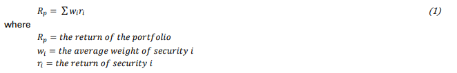
The return of a portfolio over any holding period is the weighted average of the underlying position returns and weights. If a position is held at a 1% weight and it appreciates 10% over the holding period, its contribution to return is 0.1% (1% X 10%). The sum of all individual contributions is the portfolio return, which is the weighted average of position returns:
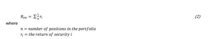
To isolate consistency, we need to level the playing field across portfolio positions by neutralizing the investor’s expression of preference for one investment over another through position weights. This can be done by assuming that each position receives the same weight. When you assume positions have the same weight, you get the portfolio’s equal-weighted return, defined as:
The equal-weighted portfolio is the simplest expression of neutrality because its weighting scheme suggests that the expected probability of some investment outcome is the same for each position. Said another way, uncertainty as to which investments will win or lose is at its maximum. The outcome has nothing to do with manager skill beyond simply selecting the investments from a wider opportunity set. To understand the connection between expected outcomes and how positions are weighted, we can look to probability and information theory.
In attempting to predict the outcome of a fair coin toss—fair in the sense that each toss is 50% likely to be heads or tails—there exists no edge to betting on one outcome over the other, despite our behavioral biases to the contrary. The chart below illustrates the amount of uncertainty as the outcome of the toss becomes more certain, either a tails or heads outcome. Notice how uncertainty (measured on the vertical axis) falls as the probability of tossing heads (moving to the right on the horizontal axis) or tails (moving to the left) increases. As uncertainty decreases, an investor should revise his bets accordingly by increasing the wager—more on this later when we discuss the weighting component of skill. But for now, our equal-weighted portfolio is evaluated as if it were a series of fair coin tosses where each position either wins or loses.

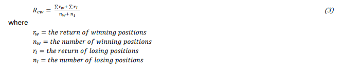
We can break out the winning and losing positions from the equal-weighted portfolio return in equation (2) as follows:
After some manipulation, we can derive the average return of winners and losers as:

Knowing the number of winning and losing positions in a portfolio is useful because it allows you to calculate a batting average. The batting average quantifies how often a manager picks winners. It is a measure of breadth of wins across the portfolio and is the yard stick for consistency.
A batting average can be generated relative to any objective—a benchmark index, a fixed return, or just whether a positive return is produced. The batting average (𝐵𝑝) can be defined for a given holding period as:

All else equal, a manager with a higher win rate will outperform one with a lower win rate.1
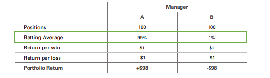
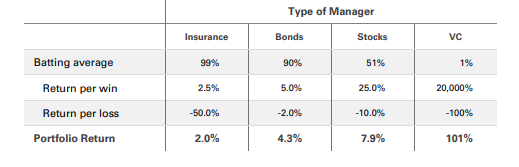
The impact of consistency in investment selection is most easily thought about in terms of its extremes—a manager that wins often, and one that loses frequently. On one extreme, Manager A in the table below implements a strategy where 99 out of 100 of her picks produce a win. Her batting average is 99%. On the other extreme, Manager B implements a strategy where 1 out of 100 of his picks produces a win. His batting average is just 1%. Given the choice between Manager A and B, most people would select Manager A, as A seems like a sure bet. This betrays an inherent bias to oversimplify complex problems. Given a batting average, most think of 100 equally placed bets, perhaps $1 each with even money odds—bet $1, win $1. In that context, Manager A would effectively double her money, while Manager B loses almost everything:
In this example the entire difference in return can be explained through the dimension of consistency. This should be intuitive given that the only variable introduced is a different batting average.
To determine the contribution to return from consistency (𝑅𝐶), we multiply the difference between the batting average and 50% with the difference between the average win and loss. 50% is important because it represents the dividing line between winning more than losing.

𝑅𝐶 is the amount of a portfolio’s return generated from winning more often than losing. All else equal, the impact of consistency improvements are linearly related to portfolio return as the batting average improvement multiplied by the difference in average wins and losses.
MAGNITUDE – WIN BY MORE THAN LOSERS LOSE
As it currently stands, our manager performance narrative is incomplete. What if the winnings do not result in equal payouts? If Manager B’s single win was a two hundred bagger—returning 20,000%—and his other positions were total losses, his return would be 101% (1% x 20,000% + 99% x -100%). Similarly, if Manager A’s wins only generated a 2.5% return and her losses were 50%, her portfolio return would be just 2.0% (99% x 2.5% + 1% x -50%). Consistency alone does not define a manager. To add to our narrative, we need to provision for the magnitude of wins versus losses.
The contribution to return from the magnitude (𝑅𝑀) of winning versus losing positions is defined as:

Here, we assume that the winning positions and losing positions have equal influence on the portfolio’s return. This again harkens back to our idea of neutrality. Assuming that a manager is equally likely to pick a winner or a loser aids in disaggregating the impact of the magnitude of wins versus losses.
Given the dimensions of consistency and magnitude, one can build intuition for how different types of investors select investments, and the risks for which they need to be aware. Extending our example above, Manager A generates small frequent wins and large periodic losses, a return profile that is similar to insurers, but which can be extrapolated to option portfolios. Insurers effectively write short put option portfolios against a wide range of risks. Their upside is known and consistent, while their downside is unknown and unlimited, but estimate-able and infrequent.
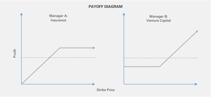
Manager B is at the opposite end of the spectrum, generating infrequent large wins and lots of small losses. This is similar to the return profile of a Venture Capital fund in which a few big wins often pay for all the failed bets in spades. At a basic level, VC’s invest in portfolios of call options with a known limited downside, but unknown, unlimited, and infrequent upside.2 It is important to note here that the return profiles of insurers and venture firms are unique corner cases on a spectrum of investment styles where more mainstream asset classes fall somewhere in the middle. I say this because, when combined, the payoff diagrams above equate to that of a simple long stock position.
That said, the return profiles of insurance and venture managers can be stylized using consistency and magnitude even though there is a strong case to be made that Venture returns are distributed according to Power Law distributions. Beyond certain limits, power law distributions have no theoretical mean or variance. This clearly poses problems within the framework presented here as the analysis is dependent on the mean, or average. This is an area that deserves a deeper dive and further research. Jerry Neumann, on his blog Reaction Wheel, has presented a compelling case that venture outcomes follow Power Law distributions.3
To the Insurance and Venture examples, I add bond and stock portfolios below. Bond portfolios generally have very high batting averages with favorable average wins to losses. Stock portfolios feature batting averages closer to 50% with favorable, but more volatile average wins to losses.
As mentioned previously, these two dimensions evaluate the impact of investment selection decisions. It turns out there is a relationship between the two. Consistency and magnitude are proportional components which sum to the equal-weighted return of the portfolio: 𝑅𝑒w = 𝑅𝐶 + 𝑅𝑀. As such, improvements in the consistency of wins can only increase return to the limit of the average win in the portfolio. In other words, consistency can only drive so much improvement. When the investor’s batting average hits the natural limit of 100%, consistency and magnitude become equal contributors to portfolio return.
All else equal, the impact of improvements in magnitude are also linearly related to portfolio return as the average of the change in wins and losses.

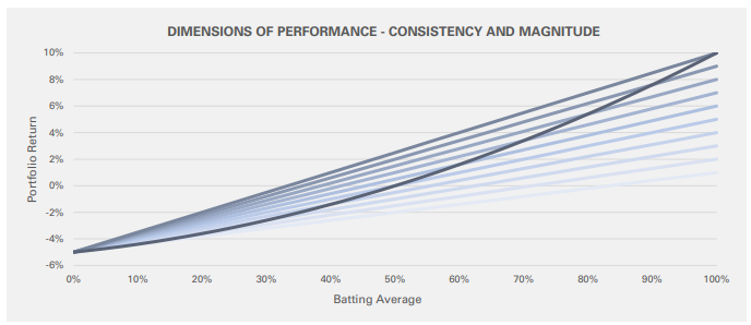
This is reflected in the following chart. The light blue lines represent improvements in the batting average (moving from left to right) given a static set of average wins and losses. For example, the highest light blue line shows the impact of a batting average improvement based on average wins of 10% versus average losses of -5%. The dark line represents improvement in both consistency and magnitude. Notice that it is non-linear, which suggests that there is leverage in simultaneous improvements in more than one dimension.
This occurs because of the symbiotic relationship between consistency and magnitude. Together they represent an investor’s skill in stock selection. Improvements in one or both will drive the portfolio’s equalweighted return 𝑅𝑒w higher.
Equations (7a) and (8a) quantify the impact from changes in consistency and magnitude individually. Realistically, that does not happen. Let’s say an investor runs an analysis and finds her batting average is poor. If she wants to improve upon it, there are two approaches. She can either attempt to select more winners— improve the numerator in her batting average—or, she can attempt to do a better job of screening out losers— lower the denominator in her batting average. Both methods, if successful, will improve her overall batting average. I refer to the latter as pruning. Just as trees periodically require removing dead branches to improve overall health, investors aught look at their processes to prune the waste.
Naturally, this has implications for concentration within portfolios. It even suggests that there is some optimal level of concentration based on a particular strategy’s batting average and magnitude.
In either case, the improvement has to capture two effects, the improvement in the batting average, and the difference in average wins versus losses from either bringing in new winners or eliminating losers. As such the combined improvement to 𝑅𝐶 and 𝑅𝑀 can be modeled as:

CONVICTION – PLAYING TO STRENGTHS
Conviction is the X factor in portfolio performance. Whereas consistency and magnitude can only be improved through the challenging exercise of better investment selection, conviction can improve performance outcomes with no additional skill in the investor’s selection abilities.
Conviction evaluates the relationship between position weights and investment outcomes. The concept is predicated on the assumption that information content is inherent in the weight of a position. This requires a departure from our previously established concept of neutrality. All else equal, a high position weight suggests greater confidence on the part of the investor in a successful investment outcome than for a lower weighted position. Unfortunately, investor confidence, conveyed through the position weight, may not always align with reality. A classic example of this calibration error would be the well-documented bias towards overconfidence in one’s decision-making abilities. A corollary is that underconfidence, or undue conservatism, can also negatively impact performance by leaving return on the table when the distribution of potential outcomes suggests being more aggressive.
Let’s say, for example, that Venture Firms A and B regularly co-invest and have decided on the same set of investments. From their own historical experience, they know that about 1/3 of investments fail to return any capital, 1/3 break even and return the invested capital, and 1/3 deliver a 200% return on capital.4 At the outset, the firms have no way to reliably differentiate between which investments will fall into each group, so they equal-weight the investments. Let’s assume that investments proceeding with additional “up” financing rounds—Series A, B, C—are more likely to persist to a successful venture exit. In the decomposition of outcomes below, Venture Firm A makes the decision to equal-weight all investments after the Series A round despite the evidence that some of those investments are more likely to be successful. The expected return for its portfolio is 78%, or 12% annualized over five years. Venture Firm B recognizes that after a successful Series A round, those investments are probabilistically more likely to be winners. The expected return for its portfolio is a significantly greater 124%, or 17% annualized.
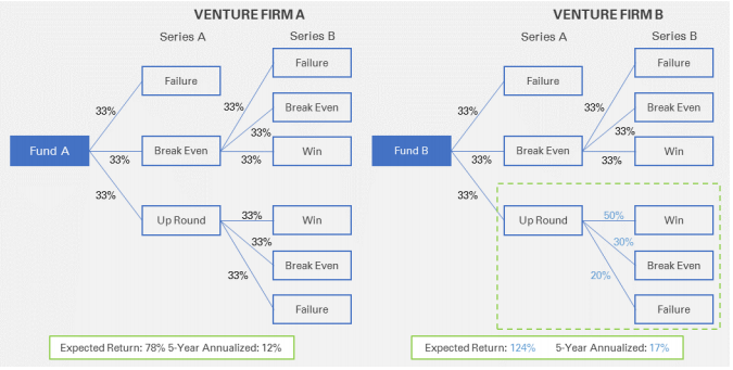
Clearly, the expected return of Firm A is significantly understated relative to Firm B, which is to say that Firm A’s portfolio construction approach likely leaves a lot of return on the table by under-allocating to winners. However, there is another subtle, but important point. Assuming investment outcomes played out as the probabilities suggest, Firm B’s portfolio would exhibit higher correlation between position weights and ex-post investment outcomes.5
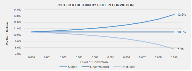
Conviction is relatively easy to define, but complicated to evaluate because it represents the convergence of portfolio construction decisions and investment outcomes. The contribution to return from the investor’s conviction (𝑅𝐾)—deviation from equal-weighting—is defined as:
In our venture example, Firm A does not deviate from equal-weighted so there would be no contribution to return from conviction. The difference in expected returns of the two firms, however, is completely explained by differences in conviction. As such, conviction can be defined even more simply as the difference between the weighted-average and equal-weighted portfolio return:

Now that we’ve defined each of the three dimensions, we find that they are additive and should sum to the portfolio return over a given holding period.

Impact attributable to conviction can result from either manager-driven portfolio construction decisions, as in our example, or spurious exogenous shocks that increase correlation between position weights and returns. For simplicity, I assume that any shocks are short-lived, independent, and mean-reverting over time, allowing us to focus on the effects of manager-driven weighting decisions.
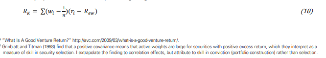
To illustrate the return impact of varying levels of conviction, I create ten hypothetical portfolios which differ only by the degree of conviction applied to the portfolio’s weights.6 The graphic below charts the position weights on the vertical axis for each portfolio from highest on the left to lowest on the right. For example, the portfolio represented by the dark blue line suggests about a 3% weight in its highest conviction position, and a 0.5% weight in its lowest conviction name.
I then introduce look-ahead bias to create three sets of randomly generated position returns.7 The returns differ only in their level of correlation with position weights. The first set is uncorrelated with position weights— correlation of 0.0. This functions as a control set whereby our expectation is that the investor’s conviction has no bearing on performance. The second set has a positive correlation with position weights of +0.1. This replicates a scenario in which an investor’s confidence is somewhat aligned with investment outcomes; she is skilled. The third set has a negative correlation with position weights of -0.1—suggestive of a manager who is overconfident in weighting decisions and is unskilled.
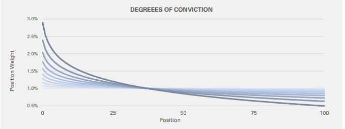
The chart below plots the portfolio return at each level of conviction for the skilled, uncorrelated, and unskilled investors. Conviction is plotted on the horizontal axis and increases from left to right. As is expected, the control portfolio with uncorrelated weights and returns delivers the same performance despite the level of conviction. The skilled manager with appropriate and realistic conviction (correlation +0.1) is progressively rewarded as his expression of conviction increases. Conversely, the unskilled manager (correlation -0.1) is penalized as his conviction/overconfidence increases.
This highlights that even slight deviations—correlation of +0.1 is not particularly large—can have a significant impact. In this case, the hypothetical portfolio with a slight positive correlation outperforms an equal-weighted portfolio by 2.7%—exact same securities, different weighting scheme. The payoff for expressing confidence is symmetric with the skilled manager outperforming by 2.7% and the unskilled manager underperforming by -2.7%.
While normal, bell-shaped distributions are great for theoretical exercises, they generally do not reflect reality. For example, if an equity investor were formulating an investment strategy and had to choose between two opportunity sets, he would likely face the choice represented in the table below. In this case he would probably always choose Option 2—higher average return, higher batting average, better magnitude in average positive versus negative return. Option 2 is statistically “skewed” in the investors favor.

From this opportunity set, an investor would then apply some conviction framework to weight the names. Option 2 differs from our hypothetical example in that it is a skewed distribution that is approximately, but not perfectly, normal. The data above is taken directly from monthly returns of US stocks from 1987-2017. Option 1 are all large stocks. Option 2 is a subset of cheap large stocks as measured by sales, earnings, and cash flows.
SO WHAT?
One useful purpose for the framework is in identifying skilled and unskilled managers within a competitive peer group. The dimensions framework quantifies the value add from investment selection (consistency and magnitude) as opposed to portfolio construction (conviction).
As we have seen, portfolios of the exact same underlying investments can yield very different performance depending on the manager’s ability to align position weights with ex-post investment outcomes expressed through conviction. One would think that managers which use a process-driven portfolio construction methodology should deliver value-add on the conviction dimension over time.
To test this thesis, I pulled positions and returns for the top 20 and bottom 20 managers from Morningstar’s U.S. Large Value and Small Value peer groups for the 5 years ending December 31, 2017.8 While an analyst could theoretically evaluate a strategy over any time frame, I look at rolling one-year periods. Public equity managers are attempting to beat indexes, and most equity indexes rebalance once annually, which aligns with a one-year buy and hold. The benchmark for the peer groups are the Russell 1000® Value and Russell 2000® Value Indexes.
To level set, below are the contributions to return by dimension for these benchmarks for the 5-year period from 2013-2017.9
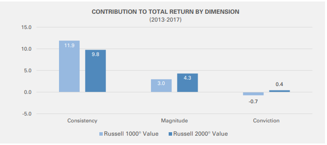
The indexes generate most of their return from consistency. Though there is no explicit empirical tie to beta, I interpret this as exposure to a broad market category—large value or small value. Magnitude is a much smaller contributor but is probably analogous to style exposures—value or growth. Conviction is the smallest contributor. As we established earlier, this contribution should only be significant in the presence of investor skill. Since the average correlation between benchmark weights and forward position returns is 0.0 for the Russell 1000® Value and Russell 2000® Value over the analysis period, it seems safe to conclude there is no “skill” implied in their cap-weighted construction.
How do professional active managers stack up? The answer is, as always, “it depends”. The scatter plot below shows the top and bottom large value managers from Morningstar. The vertical axis plots the contribution to total return over the last five years from conviction, while the horizontal axis shows consistency and magnitude (investment selection).
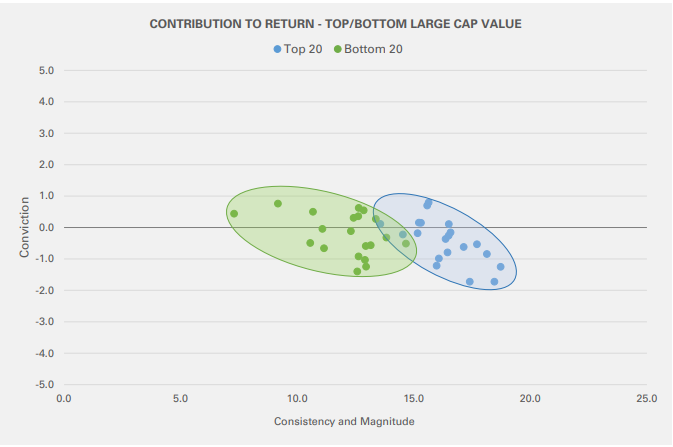
What is readily apparent in large value is that most managers, even the top ones, are not able to differentiate themselves through conviction. For the majority, the dimension is a net detractor from performance, which suggests their skill in portfolio construction is poor. In fact, most would be better off simply equal-weighting their portfolios. Notice though, that the top and bottom managers are clustered into two groups. Dots further to the right generate greater return from selection. What does it take to excel in the equity US large value space? Be a really good stock picker
It turns out though, that is not universally true across equity asset classes. Moving down capitalization to a less efficient space, small value, and the results are a bit different. The scatter plot below shows the same analysis, but on top and bottom small value universes.
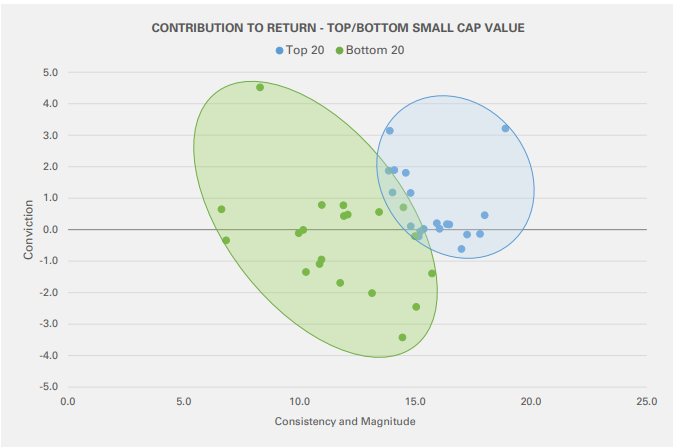
As compared to the large value chart, a few things jump out. Dispersion is much greater at the bottom end of small than large value. Large and small managers generate roughly the same amount of return from investment selection, but small value managers appear to be more skilled at portfolio construction. The majority of small value managers plot above the 0 line on conviction, suggesting portfolio construction is additive to performance.
The analysis above is by no means exhaustive. This is just one five-year period among many, and a particularly difficult one for professional managers. Future research would apply this analysis more broadly in the equity space to growth and non-U.S. managers, as well as expanding to other asset classes—fixed income, venture, and private equity portfolios.
CONCLUSIONS
This framework should be useful for both allocators and investment managers. Allocators are always seeking managers with robust processes that have the ability to deliver alpha over time. This framework provides a quantitative process whereby allocators can identify manager skill in certain areas, selection and portfolio construction. In our work studying value factors, one of the things that has surprised us is that most companies we study have negative free cash flow yield yet can still go on to produce strong investment returns. Because of this, when we see companies with strong and sustainable free cash flow, we try to figure out what structural advantages exist. Conviction is the free cash flow of manager analysis. Some managers succeed in spite of their poor skill in portfolio construction. Some managers thrive because of it. Why is this important? Because skill in conviction is all about the manager’s process, something he/she can control to amplify existing skills. Conversely, investment selection, is a wait-and-see affair.
For professional managers, the inferences from the analysis can be used to aid in refining their portfolio construction processes. While it would be impossible to suggest managers to get better at predicting the future, I do think it is fair to suggest that investors can do a better job of understanding the distributions of their own investment outcomes. If an analysis shows even mild positive correlations (+0.1), it could be a massive contributor to their advantage versus other managers. If its negative, the investor should set hubris aside and equal-weight their portfolio until they can develop a reliable and repeatable portfolio construction methodology
FOOTNOTES:
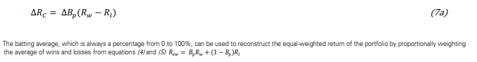
1 The batting average, which is always a percentage from 0 to 100%, can be used to reconstruct the equal-weighted return of the portfolio by proportionally weighting the average of wins and losses from equations (4) and (5): Rew = BpRw + (1-Bp)Rl
2 In both cases, insurance and venture capital, provisions are put in place by managers to tilt the odds of success in their favor. Insurers place policy limits to limit losses and Venture Capital firms insert liquidity preferences to mitigate losses on their investment. In both cases, risk is shifted to the counterparty—policyholders and founders, respectively.
3 See references to Reaction Wheel.
4 “What Is A Good Venture Return?” http://avc.com/2009/03/what-is-a-good-venture-return/.
5 Grinblatt and Titman (1993) find that a positive covariance means that active weights are large for securities with positive excess return, which they interpret as a measure of skill in security selection. I extrapolate the finding to correlation effects, but attribute to skill in conviction (portfolio construction) rather than selection.
6 The weighting scheme is determined through a decay rate meant to represent an investor’s degree of conviction in positions. Weights are determined by re-weighting the results of a formula for logarithmic decay: wi = -d ln(i) + wmax where d = a decay rate and wmax = the maximum allowable position weight
7 Returns are log-normally distributed with a mean and standard deviation of 10% and 15%, annualized. Approximately half will outperform the mean and half will underperform
8 To determine the top and bottom 20 managers, I excluded duplicate mutual fund share classes, enhanced index strategies, and strategies with greater than 500 holdings. Portfolios are reweighted to exclude cash holdings.
9 I chose this time period purposefully because it has been an exceptionally difficult period for active managers. In extending the analysis back ten years I found similar conclusions, however, the ten-year period encompasses the financial crisis which does skew the results.
REFERENCES:
Kelly, J. L., “A New Interpretation of the Information Rate”. The Bell System Technical Journal. July 1956.
Shannon, Claude E. “A Mathematical Theory of Communication.” The Bell System Technical Journal. October 1948.
Grinblatt, Mark & Titman, Sheridan, 1993. "Performance Measurement without Benchmarks: An Examination of Mutual Fund Returns," The Journal of Business, University of Chicago Press, vol. 66(1), pages 47-68, January.
Colin, Andrew. “Portfolio Attribution for Equity and Fixed Income Securities”. Chapter 5, Smoothing Algorithms. Amazon. 2014.
“Entrepreneurship and the U.S. Economy”. Bureau of Labor Statistics. https://www.bls.gov/bdm/entrepreneurship/entrepreneurship.htm
“Venture Outcome are Even More Skewed Than You Think”. VCAdventure. https://www.sethlevine.com/archives/2014/08/venture-outcomes-are-even-more-skewed-than-you-think.html
“Power Laws: How Nonlinear Relationships Amplify Results.” Farnham Street. https://www.fs.blog/2017/11/power-laws/
“Power laws in Venture”. Reaction Wheel. http://reactionwheel.net/2015/06/power-laws-in-venture.html
“Power Laws in Venture Portfolio Construction”. Reaction Wheel. http://reactionwheel.net/2017/12/power-laws-in-venture-portfolio-construction.html
“Applying Decision Analysis to Venture Investing” Clint Korver, Class 14. Kaufman Fellows Press. https://www.kauffmanfellows.org/journal_posts/applying-decision-analysis-to-venture-investing/
GENERAL LEGAL DISCLOSURES & HYPOTHETICAL AND/OR BACKTESTED RESULTS DISCLAIMER
The material contained herein is intended as a general market commentary. Opinions expressed herein are solely those of O’Shaughnessy Asset Management, LLC and may differ from those of your broker or investment firm.
Please remember that past performance may not be indicative of future results. Different types of investments involve varying degrees of risk, and there can be no assurance that the future performance of any specific investment, investment strategy, or product (including the investments and/or investment strategies recommended or undertaken by O’Shaughnessy Asset Management, LLC), or any non-investment related content, made reference to directly or indirectly in this piece will be profitable, equal any corresponding indicated historical performance level(s), be suitable for your portfolio or individual situation, or prove successful. Due to various factors, including changing market conditions and/or applicable laws, the content may no longer be reflective of current opinions or positions. Moreover, you should not assume that any discussion or information contained in this piece serves as the receipt of, or as a substitute for, personalized investment advice from O’Shaughnessy Asset Management, LLC. Any individual account performance information reflects the reinvestment of dividends (to the extent applicable), and is net of applicable transaction fees, O’Shaughnessy Asset Management, LLC’s investment management fee (if debited directly from the account), and any other related account expenses. Account information has been compiled solely by O’Shaughnessy Asset Management, LLC, has not been independently verified, and does not reflect the impact of taxes on non-qualified accounts. In preparing this report, O’Shaughnessy Asset Management, LLC has relied upon information provided by the account custodian. Please defer to formal tax documents received from the account custodian for cost basis and tax reporting purposes. Please remember to contact O’Shaughnessy Asset Management, LLC, in writing, if there are any changes in your personal/financial situation or investment objectives for the purpose of reviewing/evaluating/revising our previous recommendations and/or services, or if you want to impose, add, or modify any reasonable restrictions to our investment advisory services. Please Note: Unless you advise, in writing, to the contrary, we will assume that there are no restrictions on our services, other than to manage the account in accordance with your designated investment objective. Please Also Note: Please compare this statement with account statements received from the account custodian. The account custodian does not verify the accuracy of the advisory fee calculation. Please advise us if you have not been receiving monthly statements from the account custodian. Historical performance results for investment indices and/or categories have been provided for general comparison purposes only, and generally do not reflect the deduction of transaction and/or custodial charges, the deduction of an investment management fee, nor the impact of taxes, the incurrence of which would have the effect of decreasing historical performance results. It should not be assumed that your account holdings correspond directly to any comparative indices. To the extent that a reader has any questions regarding the applicability of any specific issue discussed above to his/her individual situation, he/she is encouraged to consult with the professional advisor of his/her choosing. O’Shaughnessy Asset Management, LLC is neither a law firm nor a certified public accounting firm and no portion of the newsletter content should be construed as legal or accounting advice. A copy of the O’Shaughnessy Asset Management, LLC’s current written disclosure statement discussing our advisory services and fees is available upon request
The risk-free rate used in the calculation of Sortino, Sharpe, and Treynor ratios is 5%, consistently applied across time
The universe of All Stocks consists of all securities in the Chicago Research in Security Prices (CRSP) dataset or S&P Compustat Database (or other, as noted) with inflation-adjusted market capitalization greater than $200 million as of most recent year-end. The universe of Large Stocks consists of all securities in the Chicago Research in Security Prices (CRSP) dataset or S&P Compustat Database (or other, as noted) with inflation-adjusted market capitalization greater than the universe average as of most recent year-end. The stocks are equally weighted and generally rebalanced annually
Hypothetical performance results shown on the preceding pages are backtested and do not represent the performance of any account managed by OSAM, but were achieved by means of the retroactive application of each of the previously referenced models, certain aspects of which may have been designed with the benefit of hindsight
The hypothetical backtested performance does not represent the results of actual trading using client assets nor decision-making during the period and does not and is not intended to indicate the past performance or future performance of any account or investment strategy managed by OSAM. If actual accounts had been managed throughout the period, ongoing research might have resulted in changes to the strategy which might have altered returns. The performance of any account or investment strategy managed by OSAM will differ from the hypothetical backtested performance results for each factor shown herein for a number of reasons, including without limitation the following:
- Although OSAM may consider from time to time one or more of the factors noted herein in managing any account, it may not consider all or any of such factors. OSAM may (and will) from time to time consider factors in addition to those noted herein in managing any account.
- OSAM may rebalance an account more frequently or less frequently than annually and at times other than presented herein.
- OSAM may from time to time manage an account by using non-quantitative, subjective investment management methodologies in conjunction with the application of factors.
- The hypothetical backtested performance results assume full investment, whereas an account managed by OSAM may have a positive cash position upon rebalance. Had the hypothetical backtested performance results included a positive cash position, the results would have been different and generally would have been lower.
- The hypothetical backtested performance results for each factor do not reflect any transaction costs of buying and selling securities, investment management fees (including without limitation management fees and performance fees), custody and other costs, or taxes – all of which would be incurred by an investor in any account managed by OSAM. If such costs and fees were reflected, the hypothetical backtested performance results would be lower.
- The hypothetical performance does not reflect the reinvestment of dividends and distributions therefrom, interest, capital gains and withholding taxes.
- Accounts managed by OSAM are subject to additions and redemptions of assets under management, which may positively or negatively affect performance depending generally upon the timing of such events in relation to the market’s direction.
- Simulated returns may be dependent on the market and economic conditions that existed during the period. Future market or economic conditions can adversely affect the returns.