The Great Inflation, Factors, and Stock Returns
By Ehren Stanhope
October 2021
“Inflation is as violent as a mugger, as frightening as an armed robber and as deadly as a hit man.” -- Ronald Reagan
Inflation is an amorphous concept that generally refers to the sustained increase in the general level of prices. Inflation has been much maligned due to the deleterious impact of the ‘Great Inflation’ era of the 1960’s and 1970’s. That period conjures images of long gas lines, commodity shortages, paltry real investment returns, and price spikes.
Since then, however, we have lived through the ‘Great Moderation’—four decades of low and decreasing inflation. Memories of the inflationary periods of the past, however, remain so visceral that signs of rising prices have recently plagued investor sentiment. Our analysis suggests that while investors are right to pay attention to inflation, comparisons with the 1970s may be overblown. Equities, as a whole, may not welcome high rates of inflation, but certain stock selection factors have shown more resilience than others in periods of rising prices.
Although Milton Friedman famously argued that “inflation is always and everywhere a monetary phenomenon”, price increases can be driven by an almost infinite set of variables. Our post-Global Financial Crisis (GFC) experience offers supporting evidence, as monetary policy has been as exceptionally loose but avoided even a brief spike above the long-run historical inflation average. In mature developed markets like Europe and Japan, even a peak above 2% would have been an achievement in retrospect. In short, loose monetary policy often precedes inflation, but is not the sole driver.
Since 1926, U.S. inflation has averaged about 3% annually. Prior to World War II (WWII), inflationary swings were common—from -10.8% (deflation) during the Great Depression to +20.1% after price controls were ended post-WWII.

The post-war era has been dominated by two global monetary regimes—the Bretton Woods system (1944-1971) and the post-Nixon Shock era (after 1971) when the last vestiges of the gold standard were released, and monetary policy became more active in the early 1980s.
The Bretton Woods Agreement in 1944 established a global monetary regime whereby the U.S. dollar was backed by gold, and other currencies were pegged to the U.S. dollar. Despite its effectiveness in restoring the global economy from the damage of WWII, by the late 1960s it gave way to a run on the dollar as economic output grew and demand for gold outstripped supply.
In 1971, Nixon removed the dollar’s exchangeability for gold and formed a new agreement—the Smithsonian Agreement—where exchange rates remained fixed to the dollar, but with no tie to gold. However, the agreement deteriorated because the dollar was overvalued. Other G10 countries preferred floating exchange rates to avoid spending their reserves on defending an inflated U.S. dollar. The era of floating exchange rates continues to this day.
The ‘Great Inflation’ Landscape
During the Great Inflation era (1965-1982), inflation annualized at 6.5%. While comparisons to our current situation are tempting, the structure of the global economy and monetary, fiscal, energy, and labor policies are dramatically different. These differences are summarized below:
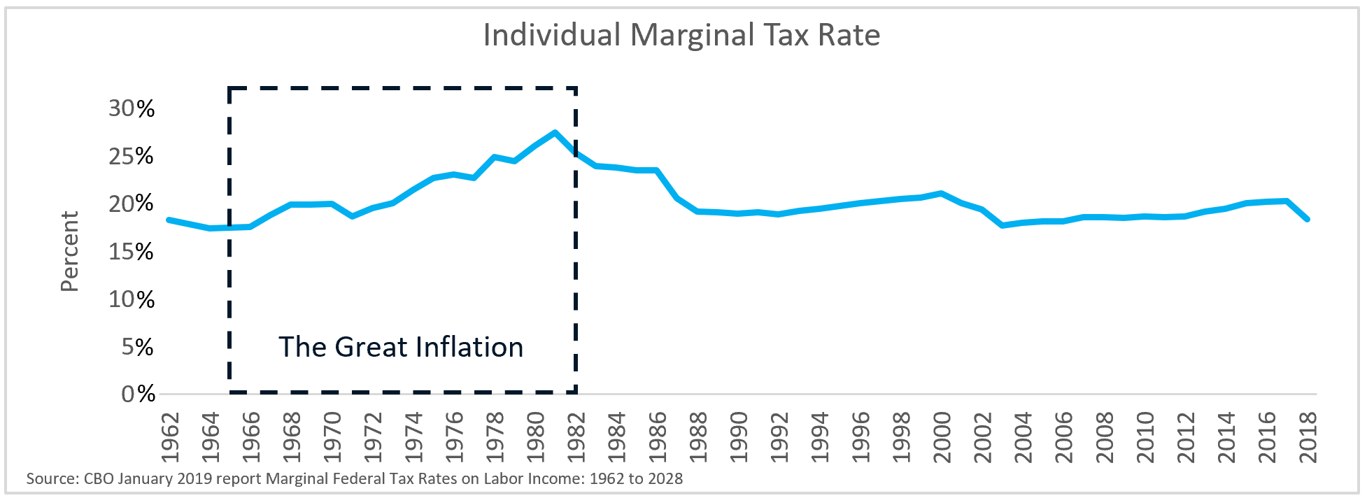
Fiscal Policy: Personal and corporate tax rates during the ‘Great Inflation’ period were considerably higher than even today’s highest expectations, contributing to a vicious inflationary cycle that looks unlikely to repeat.
The Employment Act of 1946 established that the federal government was responsible for achieving maximum employment and maintaining purchasing power (the origination of the FOMC’s dual mandate). Years of policies targeting full employment had ignored price pressures. Fiscal budget deficits for funding President Johnson’s ‘Great Society’ initiative and the Vietnam War were the highest since FDR’s New Deal.
Personal tax rates were high and there were no cost-of-living adjustments for individual income tax brackets prior to 1978. This pushed workers into higher tax brackets—exacerbating the ‘stagflation’ (high inflation, low economic growth) aspect of the Great Inflation era. Though workers were garnering a higher share of corporate profits through collective bargaining (discussed further in Labor section below), tax creep was taking an ever-increasing share of those gains. Between 1965 and 1980, the average individual marginal tax rate rose 57%!
Corporate taxes were high—averaging 48% from 1965-1982. High tax rates under high inflation regimes exacerbate inflationary forces by promoting corporate conspicuous consumption. Consider a company generating $1,000 per year in revenues with $100 in earnings. At a 48% tax rate, it pays $48 in taxes for a $52 after-tax profit. Now, let’s assume a 10% rate of inflation.
Without getting into the extreme minutiae of inflation adjustments, it’s important to note that inflation is broadly a 'tax' on cash coming in, i.e. revenues, not profits. Applying a 10% rate of inflation to our simple example virtually wipes out profits.
High tax rates within high inflation regimes can push the effective tax rate well above 100%! In such an extreme situation, it behooves corporations to rack up expenses to reduce pre-tax profits. Below is an illustration of what the effective tax curve looks like for a company with a 10% profit margin under 48% and 26.5% tax regimes.1
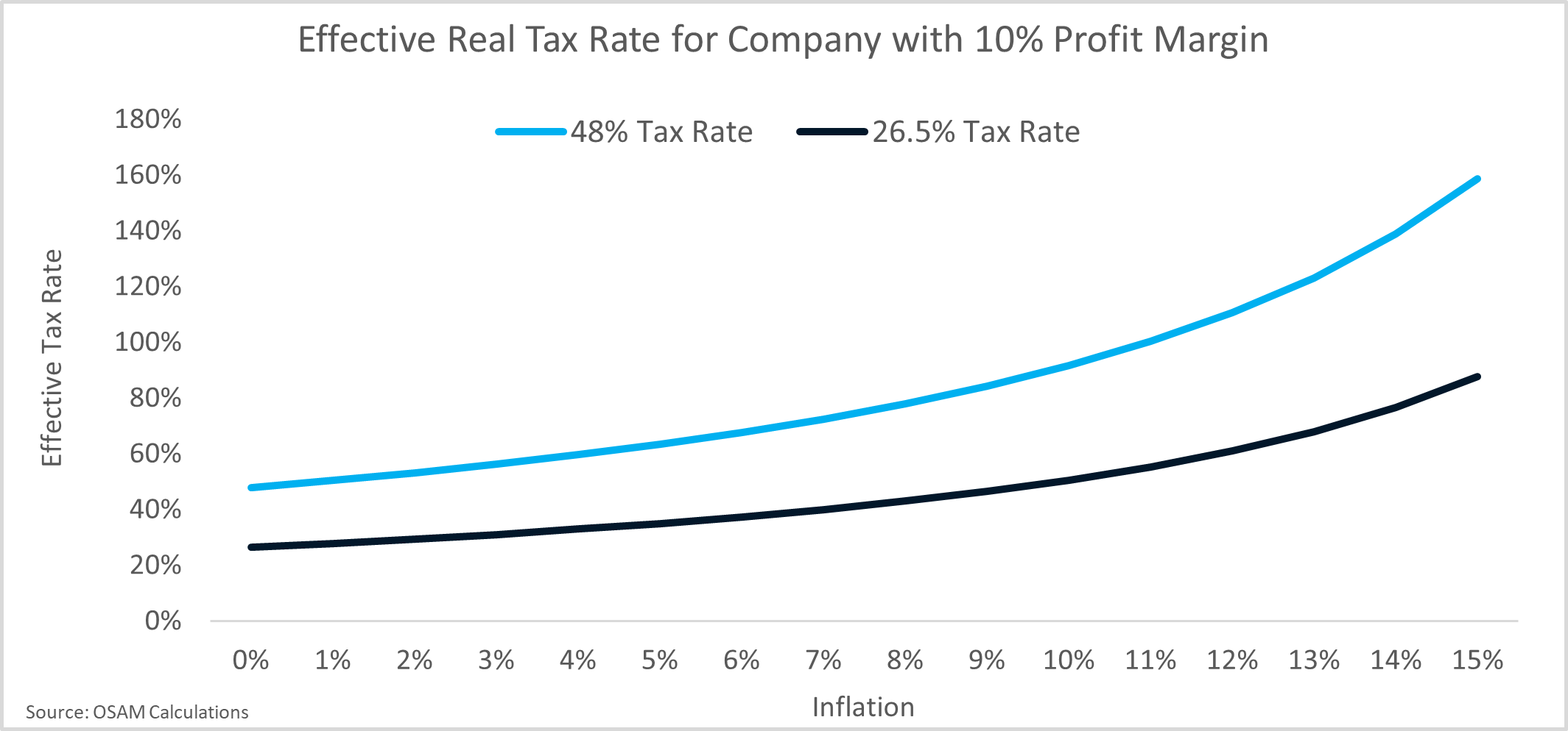
The key takeaway and key difference between the 1970s and today is that the slope and level of the 48% curve is much higher and steeper than what we face today even under an aggressive 10% inflation assumption. In short, current corporate tax rates should not exacerbate inflationary forces.
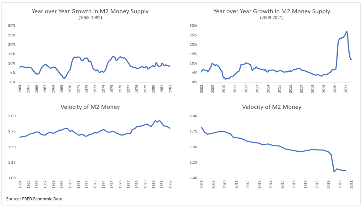
Monetary policy: Although the money supply has grown at a similar rate as in the ‘Great Inflation’, the velocity of money has remained sluggish in recent years, mitigating the risk of an inflationary spike.
Believing that there was a tradeoff between employment and inflation (the Philips Curve), central bankers tolerated the 'cost' of higher inflation for the 'benefit' of full employment. Year-over-year growth in the supply of money (M2) averaged 8.7% from 1965-1982. Since 2008, M2 has grown at an average 7.6%. While the similarities are striking, it should be noted that the velocity of money accelerated during the Great Inflation and has done the opposite in the post-GFC world—which is to say the system is currently awash with liquidity that is not being used.2
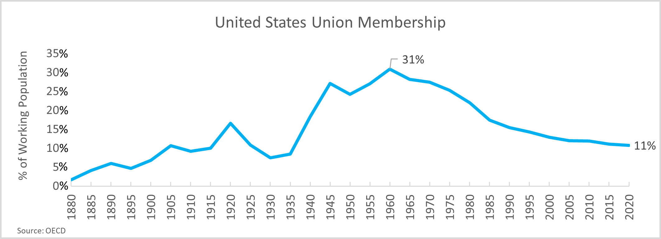
Labor – The 1950s and 1960s were the heyday for organized labor as union membership grew rapidly after the Great Depression due to New Deal legislation. Strong collective bargaining and rising wages fueled economic growth and inflation. There is a flywheel that can perpetuate the growth of wages and inflation, notably at full employment. Rising wages fuel demand for products and services, which pushes up prices, which pushes up labor’s demand for wage increases, etc. Union membership has fallen to approximately 1/3 of its 1960 peak, employment remains a weak spot in the post-pandemic era, and record job openings are available. For the time being, there is a lot of slack in the labor market.
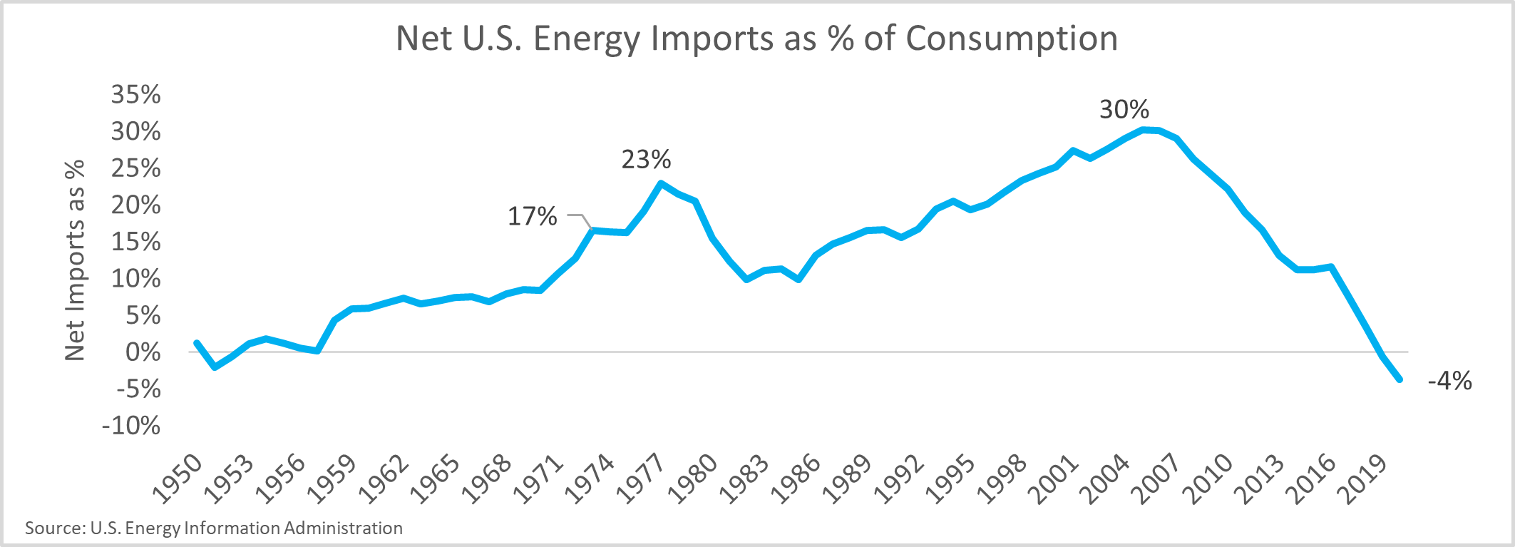
Energy – 1973 featured the 1st major oil shock due to an oil embargo proclaimed by Saudi Arabia. At the time, U.S. net energy imports accounted for 17% of total energy consumption, peaking just shy of the second oil shock in 1979 at 23%. Due to the shale revolution, the U.S. is now a net exporter of energy and more protected from commodity shocks.
Policy Summary – During the Great Inflation, a combination of easy monetary policy, a massive pivot in the global exchange rate regime, a tight labor market featuring strong labor negotiation power, high corporate tax rates, and a commodity shock all conspired to send inflation surging. Since Paul Volker 'broke the back' of inflation with decisive action, inflation has largely oscillated between 1 and 5% in what is known as the ‘Great Moderation’.3
Historical Investment Impact
Defining Inflation Regimes
While we do not believe that rampant pro-longed inflation is imminent, it is possible. The key question for investors is how inflation will impact their portfolios. We use the Consumer Price Index (CPI) index as a proxy for inflation. CPI reflects changes in weighted average prices for a basket of goods and services over time—prices of food, clothing, shelter, fuels, transportation, doctors’ and dentists’ services, drugs, and other goods and services that people buy for day-to-day living. The index has many flaws, but the CPI is widely available and the most watched inflation gauge.
There are two ways of thinking about inflation—expected and unexpected inflation. As the name suggests, expected inflation is inflation that investors anticipate and comes to fruition. While expected inflation can be planned for, unexpected inflation cannot. Unexpected inflation can occur to the upside or downside. In accelerating inflationary environments, unexpected inflation might be an expectation for 3%, but actual inflation of 5%, or an expectation of 3% that comes in at 1%. The challenge with unexpected inflation is that it is very difficult to measure historically. Today, we can look at the difference in yield between nominal Treasuries and Treasury Inflation Protected Securities (TIPS) as a proxy for expected versus realized inflation, but unfortunately, that data only begins in 1997. After exploring various definitions of inflation, we settled on the trailing 12-month change in CPI that is coincident with the returns evaluated.
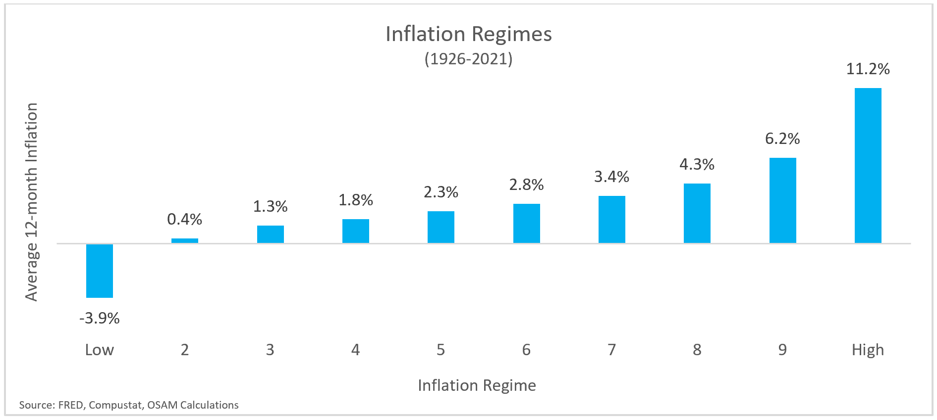
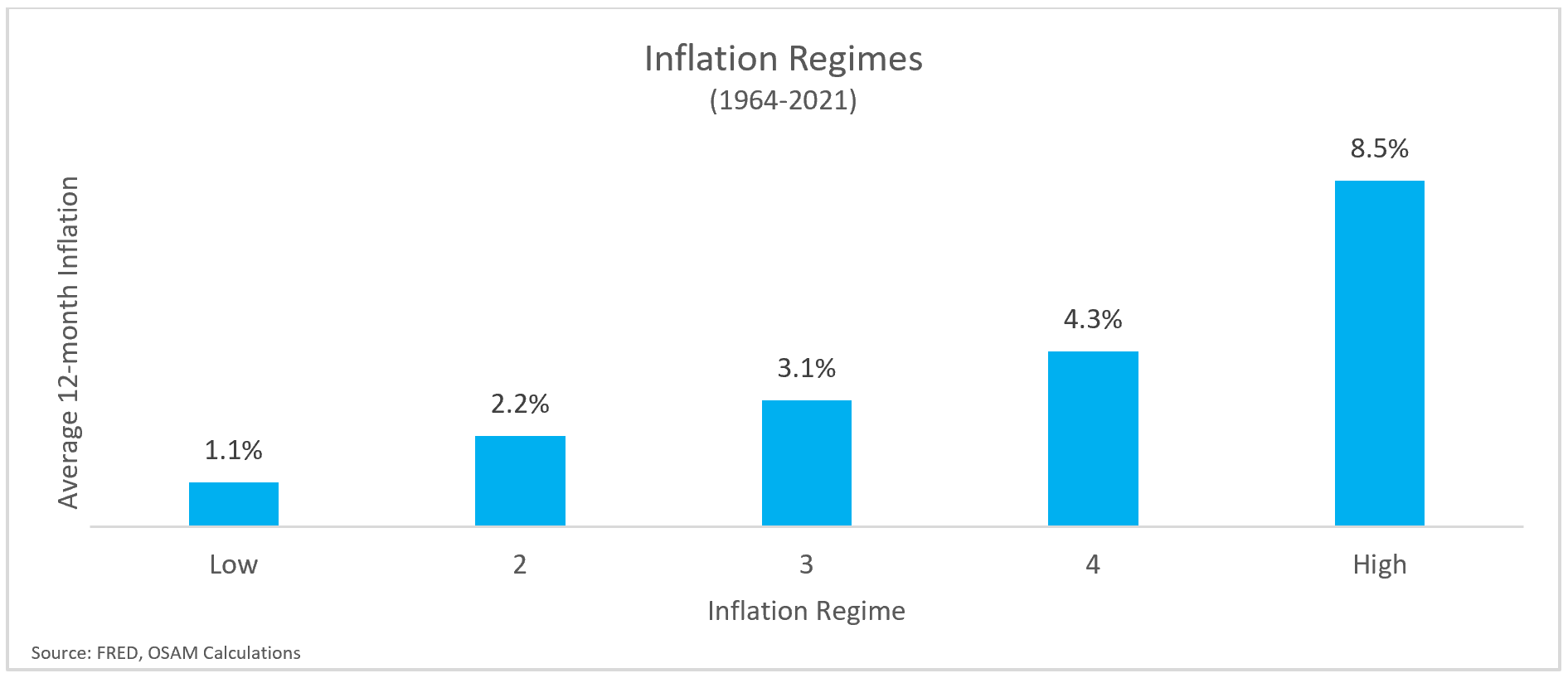
We calculated the rolling 12-month rate of inflation as of each month between January 1926 - June 2021 and then divided the observations into 10 decile groups (Inflation Regimes) based on the level of inflation. The chart below shows the average rate of inflation for each regime.
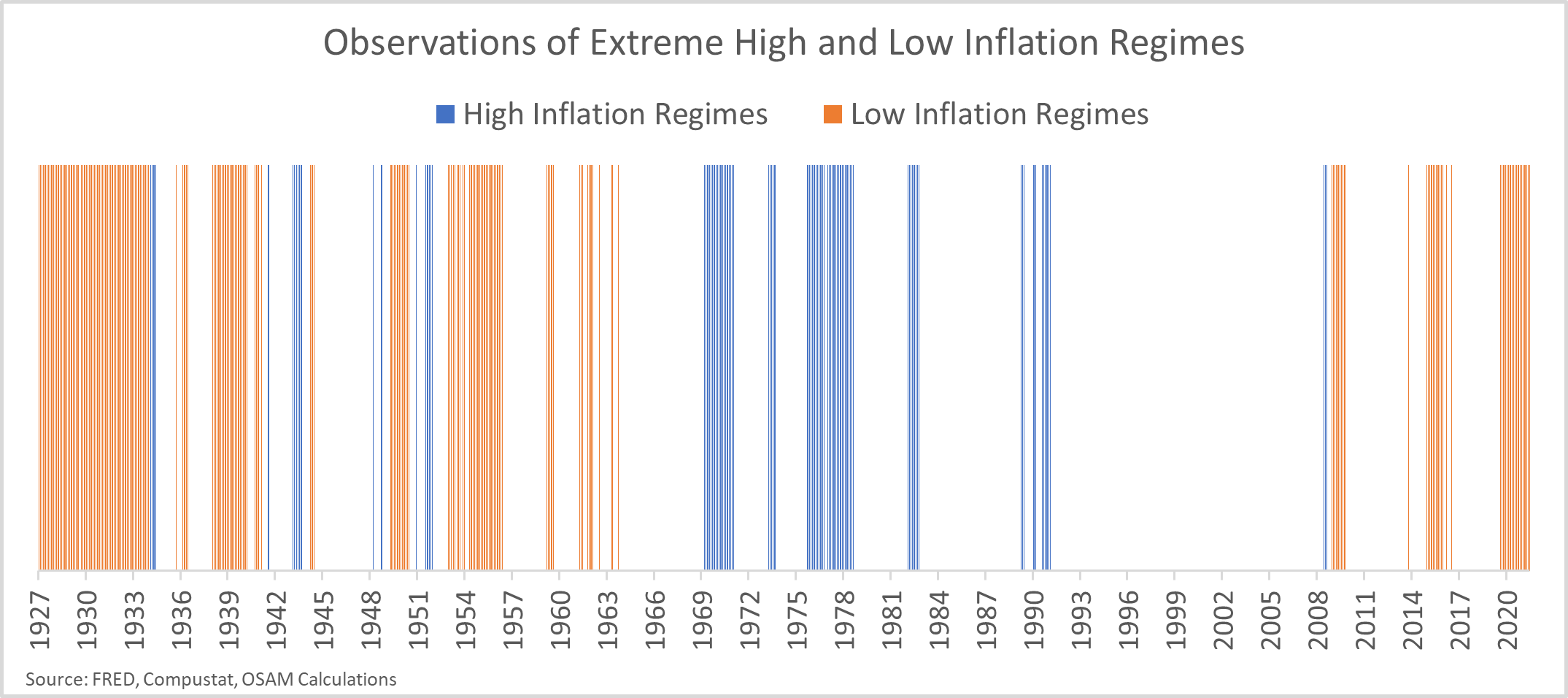
Each regime contains observations from multiple different decades. For example, the leftmost column (Low) includes observations ending in the 1920s, 1930s, 1940s, 1950s, and 2000s. The chart below shows the instances of extremes—high and low inflation. One interesting observation is that investors are concerned about runaway inflation, even though we are currently in—and have been in—the most deflationary decile more often since the 2008 crisis than in the six decades prior.
Equity Market Performance in Inflation Regimes
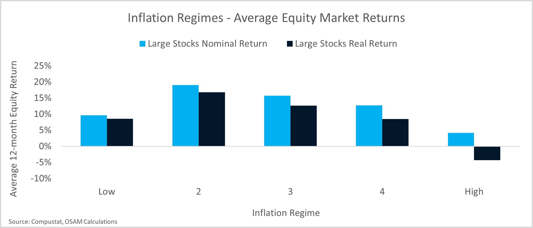
We measure the average of 12-month equity market returns (nominal and real) corresponding to the ten Inflation Regimes. Equities tend to struggle at the extremes—on a nominal and real basis. The goldilocks environment in regimes 4 and 5 corresponds to an inflation rate of roughly 2%, give or take.

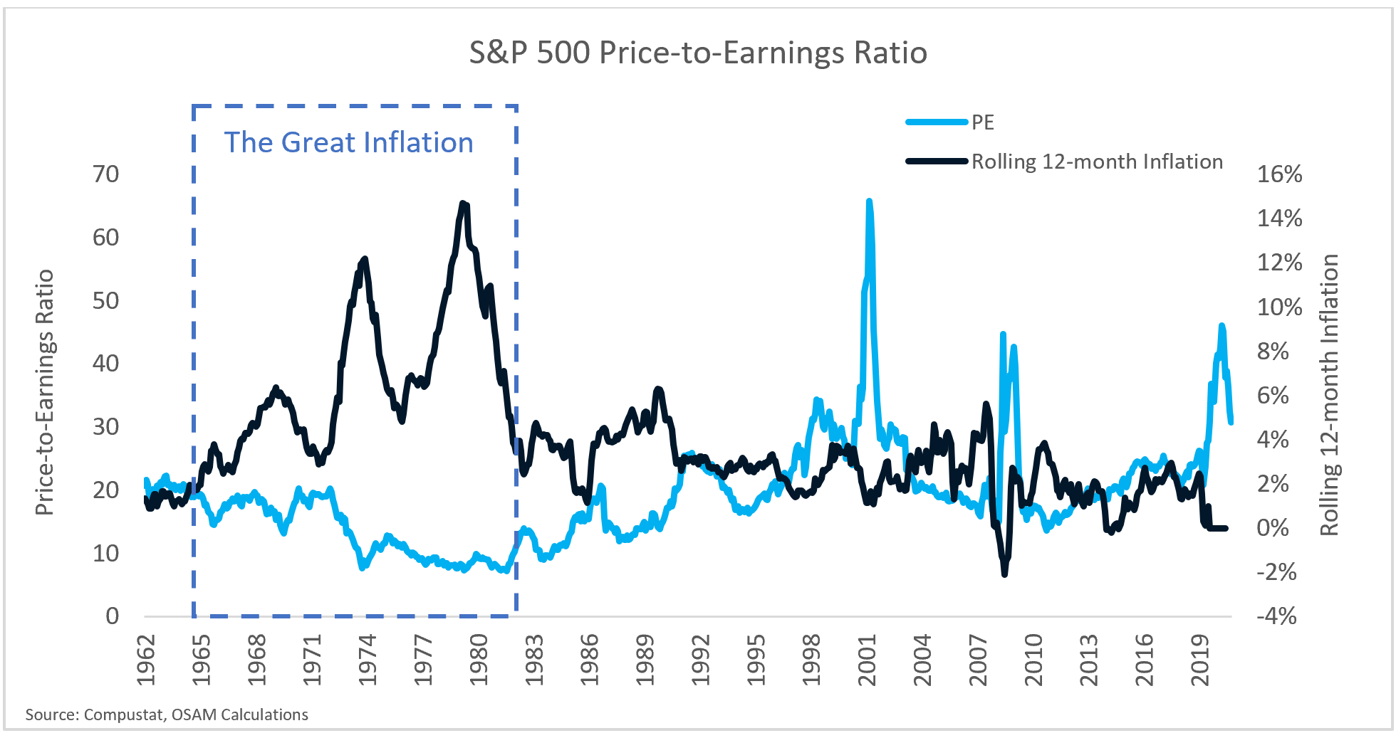
This data supports the widely held belief that high inflation regimes beget lower equity market returns. In the high inflation regime, nominal equity returns are the second lowest (outperforming only the most deflationary environments) and the lowest in real terms. As inflation climbs, equity returns fall. This often stems from 'multiple compression'. During the Great Inflation, the S&P 500 price-to-earnings (PE) ratio shrank from roughly 20x in 1965 to 10x in 1982, meaning that investors required greater returns for the risk of allocating to equities when inflation raged.
Factor Performance in Inflation Regimes
Next, we review excess returns in a U.S. Large Stocks universe for the cheapest, highest-yielding, and highest-ranked deciles of our Value, Shareholder Yield, and Momentum themes from 1926 to 2021, respectively.4 Note that Shareholder Yield consistently outperforms across all regimes, particularly in higher inflation environments. The disparity between factors in the lowest inflation regime is similarly interesting. The -3.9% average inflation rate captures deflationary environments. While Shareholder Yield and Momentum hold up quite well, Value struggles. This is likely due to the observations in that regime from the 1920s and 1930s, when cheap Utility stocks performed particularly poorly and value’s recent struggles since the GFC.5
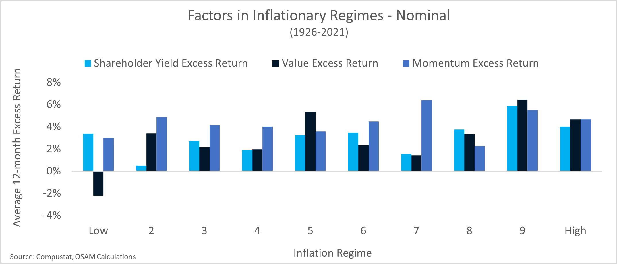
The results for selection factors beg the question, why might factors do well in high inflation environments? There are several potential explanations.
Value
Theoretically, a firm’s market capitalization is the market’s estimation of the present value of all its future cash flows. Value stocks typically generate most of that value in near-term cash flows. Growth stocks tend to be 'long duration' assets, meaning cash flows further out into the future represent a disproportionate share of their market cap. Long-duration assets are more sensitive to rising discount rates, and investors widely believe that such longer duration assets (growth stocks) do poorly when rates rise. That said, rising inflation often begets rising interest rates as central banks try to quell inflationary pressures. There was some evidence of this explicit relationship during the COVID recovery, but it is inconsistent over longer time periods.
We noted earlier that inflationary periods tend to suppress PE multiples at the aggregate market level. Value stocks have an advantage because their multiples are already low, minimizing the impact of compression relative to growth stocks.
Momentum
As we discuss in Factors from Scratch, price momentum tends to be pretty good at identifying earnings growth in advance.6 In an environment where price pressures are strong and profit margins are falling, rapidly growing earnings indicate an ability to pass on those inflationary costs and grow future cash flows in excess of inflation. When facing inflation headwinds, this is a powerful cocktail.
Shareholder Yield
Shareholder Yield is the combination of dividends and share buybacks, which represent the return of capital to shareholders. Stocks with strong Shareholder Yield have two features making them advantageous in inflationary periods:
- Stocks with strong Shareholder Yield tend to trade in about the cheapest 1/3 by valuation. As a result, they get a tailwind from the same explanations highlighted above for value stocks.
- There is a corollary to the duration argument that is only applicable to stocks with strong Shareholder Yield. Shareholder Yield is usually dominated by the buyback component of the signal. Once announced, buyback programs typically last for 12-18 months and represent a large upfront cash distribution to investors (on top of dividends). If Value stocks benefit from being 'short duration', then stocks with strong Shareholder Yield have buyback-driven cash outlay that shortens duration even further.
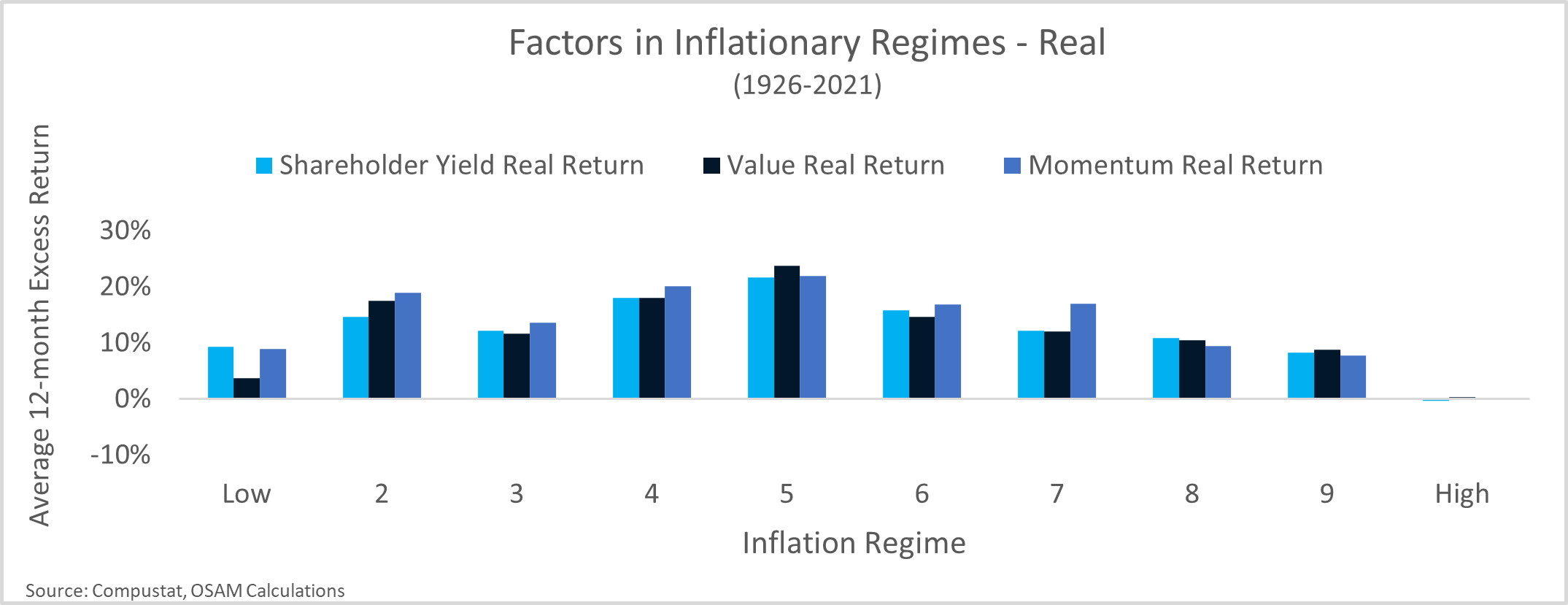
From the perspective of inflation-adjusted real returns, we see a similar pattern. However, in the highest inflation regime—11.2% average annual inflation—the excess return associated with factors allows equity investors to just keep pace with purchasing power.7 Recall that in the highest inflation regime the equity market generally delivered negative real returns. This regime only occurs about 10% of the time, but factors serve as a key hedge within equity portfolios in those runaway inflation environments.
Key Takeaways
So, is inflation really a mugger? An armed robber? As deadly as a hit man? For equity investors, it might just be possible to reduce inflation to an amateur pickpocket. As the inflation debate rages on, there are a few key points to consider for structuring portfolios.
The Great Inflation was a bit of a historical aberration by length and magnitude. In hindsight, many policies were aligned to fuel inflation. Fiscal and monetary policymakers feared sacrificing full employment at the altar of inflation, allowing loose monetary policy to reign supreme. High tax rates during a time of high inflation incentivized conspicuous corporate consumption. Labor’s strong negotiating power caused an upward thrust in wages that fed the wage/price flywheel ever higher. Finally, a reliance on energy imports left the economy susceptible to shocks. Though these points are all U.S. specific, there is a direct link to non-U.S. inflation that is primarily tied to global reliance on the U.S. dollar and dollar-priced commodities, like oil.
While nobody knows whether the recent price spikes will produce sustained inflation, we know that the previous episode of sustained higher inflation was structurally very different from today’s environment. We can draw inference from the era to key in on what to watch out for—strong employment and wage increases, an increase in the velocity of money, and policy preference to let inflation run high.
As we dive into the impact on equity markets, there does appear to be a link between high inflation and lower equity returns, most likely associated with a compression in valuations that occurs, as it did during the Great Inflation. That said, certain factors, like Value, Momentum, and Shareholder Yield, historically hold up quite well in moderate-to-high inflation regimes.
Footnotes
1 The most recent rate discussed under the Biden Tax Plan
2 The velocity of money is the ratio of nominal gross domestic product to the money supply.
3 Many economists and historians also credit the pivot to supply-side economics, particularly in the U.S. and U.K., as a major contribution to the reduction in global inflation.
4 Each factor is constructed within an equal-weighted universe of Large U.S. Stocks using CRSP/Fama French data prior to 1964 and Compustat after 1964.
5 https://osam.com/Commentary/value-is-dead-long-live-value
6 https://osam.com/Commentary/factors-from-scratch
7 A 0% real return suggests no change in purchasing power and returns simply matching realized inflation over the period.
Appendix A: Results For Quality Factors
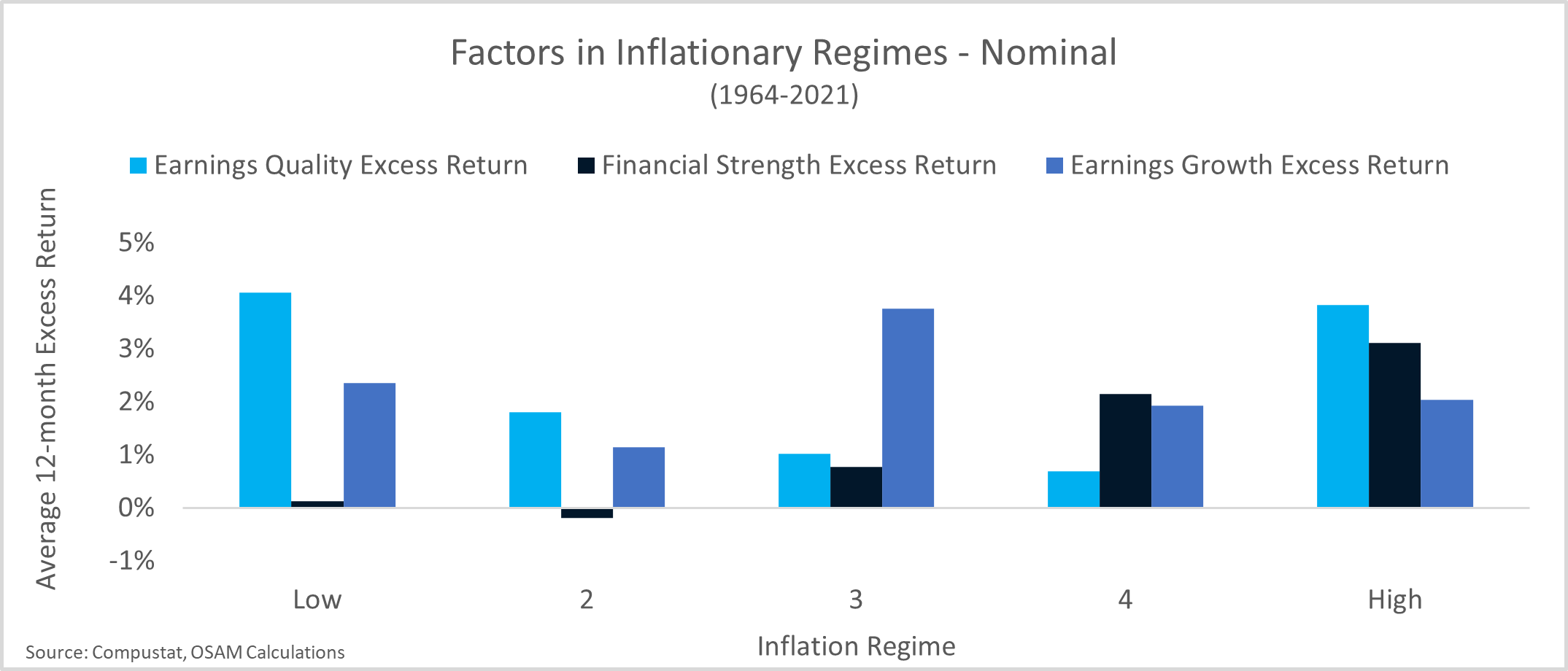
We narrowed the inflation research to the 1964-2021 timeframe to assess inflation’s impact on quality factors due to the availability of data. Quality themes tend to be more granularly defined and the data back to 1926 is lacking. Because the number of observations decreased, we evaluate inflation regimes in quintiles to keep the number of underlying observations roughly consistent.
We think of quality from three perspectives—Earnings Quality, Financial Strength, and Earnings Growth. Earnings Quality evaluates the conservativism of accounting choices and capital allocation. Financial Strength measures the reliance on outside sources of capital to support the balance sheet. Earnings Growth evaluates the health of the underlying business through margins, free cash flow trends, and returns on capital.
The chart below displays the excess returns of quality factors. We find that stocks with strong Earnings Quality perform well in both low and high inflation regimes. Earnings Growth follows a similar, though less-clear, pattern. Stocks with strong Financial Strength tend to outperform as inflation increases.

O’SHAUGHNESSY ASSET MANAGEMENT, L.L.C. CANVAS® PLATFORM IMPORTANT DISCLOSURES
CANVAS® is an interactive web-based investment tool developed by O’Shaughnessy Asset Management, L.L.C. (“OSAM”) that permits an investment professional (generally a registered investment advisor or a sophisticated investor) to select a desired investment strategy for the professional’s client. At all times, the investment professional, and not OSAM, is responsible for determining the initial and ongoing suitability of any investment strategy for the investment professional’s underlying client. The professional’s client shall not rely on OSAM for any such initial or subsequent review or determination. Rather, to the contrary, at all times the professional shall remain exclusively responsible for same. See MORE ABOUT CANVAS below and Release and Hold Harmless at the end of this Important Disclosure Information.
Reliance on Investment Professional: OSAM has relied, and shall continue to rely, on the investment professional’s knowledge and experience to understand the inherent limitations of the performance presentation, including those pertaining to back-tested hypothetical performance. All performance presentations, including hypothetical performance, are the direct result of the investment professional’s request, independent of OSAM. Depending upon the investment professional’s direction and selection, hypothetical presentations can include both OSAM and non-OSAM Models and/or strategies. The below discussion as to the material limitations of back-tested hypotheticals apply to both OSAM and non-OSAM Models and/or strategies.
Intended Recipient: CANVAS content is intended for the investment professional only not to be shared with an underlying client unless in conjunction with a meeting between the investment professional and its client in a one-on-one setting. OSAM assumes that no hypothetical performance-related content will be provided directly to the professional’s client without the accompanying consultation and explanation of the professional. The content is intended to assist the professional in evaluating the appropriate investment strategy for the professional’s client.
OSAM Models. OSAM has devised various investment models (the “Models”) for CANVAS, the objectives of each are described herein. The investment professional is not obligated to consider or utilize any of the Models. As indicated above, at all times, the investment professional, and not OSAM, is responsible for determining the initial and ongoing suitability of any Model for the investment professional’s underlying client. Model performance reflects the reinvestment of dividends and other account earnings and are presented both net of the maximum OSAM’s investment management fee for the selected strategy and gross of an OSAM investment management fee. Please Note: As indicated at Item 5 of its written disclosure Brochure, OSAM’s CANVAS management fee ranges from 0.20% to 1.15%. The average percentage management fee for all CANVAS strategies is 0.36%. The percentage OSAM management fee shall depend upon the type of strategy and the corresponding amount of assets invested in the strategy; generally, the greater the amount of assets, the lower the percentage management fee. Please Also Note: The performance also do not reflect deduction of transaction and/or custodial fees (to the extent applicable), the incurrence of which would further decrease the performance. For example, if reviewing a strategy with a ten-year return of 10.0% each year, the effect of a 0.10% transaction/custodial fee would reduce the reflected cumulative returns from 10.0% to 9.9% on a 1 year basis, 33.1% to 32.7% on a 3 year basis, 61.1% to 60.3% on a 5 year basis and 159.4% to 156.8% on a 10 year basis respectively.. Please Further Note: Transaction/custodial fees will differ depending upon the account broker-dealer/custodian utilized. While some broker-dealers/custodians do not charge transaction fees for individual equity (including ETF) transactions, others do. Some custodians charge fixed fees for custody and execution services. Choice of custodian is determined by the investment professional and his/her/its client. Higher fees will adversely impact account performance.
OSAM does not maintain actual historical performance results for the Models. In order to help assist the investment professional in determining whether a Model is appropriate for the professional’s client, OSAM has provided back-tested hypothetical (i.e., not actual) performance for the Model. OSAM, with minor deviations that it does not consider to be material*, currently uses the Models (i.e., live models vs. the reflected back-tested versions thereof) to manage actual client portfolios (see Model Deviations below). The performance reflects the current Model holdings, which are subject to ongoing change.
Material Limitations: The Performance is subject to material limitations. Please see Hypothetical/Material Limitations below. During any specific point in time or time-period, the Models, as currently comprised, performed better or worse, with more or less volatility, than corresponding recognized comparative indices, benchmarks or blends thereof.
Past performance may not be indicative of future results. Therefore, it should not be assumed that future performance of any specific investment or investment strategy (including the Models), will be profitable, equal any historical index or blended index performance level(s), or prove successful. Historical index results do not reflect the deduction of transaction and custodial charges, or the deduction of an investment management fee, the incurrence of which would have the effect of decreasing indicated historical performance results. The Russell 3000 is a market capitalization-weighted index of 3000 widely held large, mid, and small cap stocks. Russell chooses the member companies for the Russell 3000 based on market size and liquidity. The MSCI All Country World Index is a market capitalization weighted index designed to provide a broad measure of equity-market performance throughout the world. The MSCI is maintained by Morgan Stanley Capital International and is comprised of stocks from 23 developed countries and 24 emerging markets. The Barclays Capital Aggregate Bond Index is a market capitalization-weighted index, meaning the securities in the index are weighted according to the market size of each bond type. Most U.S. traded investment grade bonds are represented. Municipal bonds and Treasury Inflation-Protected Securities are excluded, due to tax treatment issues. The index includes Treasury securities, Government agency bonds, Mortgage-backed bonds, corporate bonds, and a small amount of foreign bonds traded in U.S. The historical performance results for the Russell 3000, MSCI and Barclays are provided exclusively for comparison purposes only, to provide general comparative information to help assist in determining whether a Model or other type strategy (relative to the reflected indices) is appropriate for his/her investment objective and risk tolerance. Please Also Note: (1) Performance does not reflect the impact of client-incurred taxes; (2) Neither Model or the selected strategy holdings correspond directly to any such comparative index; and (3) comparative indices may be more or less volatile than the Model or selected strategy.
Hypothetical/Material Limitations-performance reflects hypothetical back-tested results that were achieved by means of the retroactive application of a back-tested portfolio and, as such, the corresponding results have inherent limitations, including: (a) the performance results do not reflect the results of actual trading using investor assets, but were achieved by means of the retroactive application of the Model or strategy (as currently comprised), aspects of which may have been designed with the benefit of hindsight; (b) back tested performance may not reflect the impact that any material market or economic factors might have had on OSAM’s (or the investment professional’s) investment decisions for the Model or the strategy; and, correspondingly; (c) had OSAM used the Model to manage actual client assets (or had the investment professional used the selected strategy to manage actual client assets) during the corresponding time periods, actual performance results could have been materially different for various reasons including variances in the investment management fee incurred, transaction dates, rebalancing dates (increases account turnover), market fluctuation, tax considerations (including tax-loss harvesting-increases account turnover), and the date on which a client engaged OSAM’s investment management services.
MORE ABOUT CANVAS®
CANVAS is an interactive web-based investment tool developed by O’Shaughnessy Asset Management, L.L.C. (“OSAM”) that permits an investment professional (generally a registered investment advisor or a sophisticated investor) to select a desired investment strategy (the “Strategy”) for the professional’s client. At all times, the investment professional, and not OSAM, is responsible maintaining the initial and ongoing relationship with the underlying client and rendering individualized investment advice to the client. In addition, the investment professional and not OSAM, is exclusively responsible for:
- determining the initial and ongoing suitability of the Strategy for the client;
- devising or determining the specific initial and ongoing desired Strategy;
- monitoring performance of the Strategy; and,
- modifying and/or terminating the management of the client’s account using the Strategy.
Hypothetical Limitations: To the extent that the investment professional seeks for CANVAS to provide hypothetical back-tested performance, material limitations apply-see above.
Model Deviations: As indicated above, OSAM, with minor deviations that it does not consider to be material*, currently use the Models to manage actual client portfolios (i.e., the live Models). The deviations include:
- the use of proxies if and when an ETF used in the back-test was not available*. While the back-tested and live strategies both utilize the same investment themes, back-tested proxies can deviate from live models based on limitations of historical information;
- back-tested data presented utilizes a month-end rebalance while actual live model performance reflects intra-month rebalances;
- OSAM, as a discretionary manager, can update its live models as determined necessary. These changes will then be applied retroactively to back-tested models, the resulting performance of which would be different than that of the actual historical models-see Hypothetical/Material Limitations above; and,
- Financial statement information may be restated over time, which information was not reflected in the historical back-tested models. Companies will also have mergers and acquisitions or other corporate events that can retrospectively affect the names and corporate identities of organizations in the historical back-tests. Data providers providing pricing and return information may update historical data upon discovering deficiencies or omissions.
Strategy Sampling Impact: The implementation of OSAM strategies utilize a sampling of the underlying individual Strategy positions, and, as the result thereof, the underlying securities’ weighting could unintentionally deviate +/- the Strategy allocation target OSAM calculates the CANVAS fees based on the mix of strategies that are utilized at the establishment of the account. Therefore, the sampling approach can cause deviations between the CANVAS strategy allocation establishment (and its corresponding fee) and the implementation of that CANVAS strategy.
ESG Portfolios/Socially Responsible Investing Limitations. To the extent applicable to the strategy chosen by the investment professional, Socially Responsible Investing involves the incorporation of Environmental, Social and Governance considerations into the investment due diligence process (“ESG). There are potential limitations associated with allocating a portion of an investment portfolio in ESG securities (i.e., securities that have a mandate to avoid, when possible, investments in such products as alcohol, tobacco, firearms, oil drilling, gambling, etc.). The number of these securities may be limited when compared to those that do not maintain such a mandate. ESG securities could underperform broad market indices. Investors must accept these limitations, including potential for underperformance. Correspondingly, the number of ESG mutual funds and exchange-traded funds are few when compared to those that do not maintain such a mandate. As with any type of investment (including any investment and/or investment strategies recommended and/or undertaken by OSAM), there can be no assurance that investment in ESG securities or funds will be profitable, or prove successful.
Tax Management Function: When requested by the investment professional, OSAM will use best efforts to work within Onboarding Budgets, Annual Tax Budgets, and Tracking Error Budgets. However, market and/or specific stock price fluctuations can occur quickly and can correspondingly adversely affect our ability to manage to specified budgets. Additionally, changes to tax budgets, cash flows in and out of an account, mandatory corporate actions, and funding with securities can also impact preciseness. The investment professional must accept this risk. In addition:
- OSAM has not, and will not, verify the accuracy of any tax-related information provided;
- In the event that any such information provided is inaccurate or incomplete, the corresponding results will be inaccurate or incomplete;
- Tracking Error Budgets are relative to the Model, not the benchmark;
- OSAM is not a CPA and this is not tax advice;
- Tax laws and rates change;
- While we seek to follow the investment professional prescribed target models, ranges, timeframes, tax budgets, and seek not to create wash sales or exceed expected tax budgets, there can be no assurance that the CANVAS tool will be able to accurately do so; and,
- For specific personalized tax-related advice, consult with a CPA or other tax professional.
Fixed Income ETF Model-The models are constructed using passive fixed income ETFs. The models attempt to target varying levels of duration and credit exposure relative to the Barclays Aggregate Index. The expense ratios of the underlying ETF’s are born by the investor and are separate and apart from CANVAS related fees.
Miscellaneous Limitations/Issues:
- Results in the Transition Portal reflect expense ratios corresponding to the specific funds indicated/provided by the investment professional. Expense ratios are provided by an unaffiliated database. Results also reflect projected future yields corresponding to such current indicated funds. Such data may not be precise;
- The risk-free rate used in the calculation of Sortino, Sharpe, and Treynor ratios is 5%, consistently applied across time;
- OSAM did not begin to offer CANVAS until April 2019. Prior to 2007, OSAM did not manage client assets; and,
- A copy of OSAM’s written disclosure Brochure, Form CRS and Privacy Notice remains available on this CANVAS website or at www.osam.com.
Release and Hold Harmless
The professional, to the fullest extent permitted under applicable law, agrees to release, defend, indemnify and hold OSAM (including its officers, directors, members, owners, employees, agents, and affiliates) harmless from any and all adverse consequences, financial or otherwise, of any type or nature arising from or attributable to the professional’s access to, and use of, CANVAS, including, but not limited to, any claims for alleged or actual client losses or damages of any kind or nature whatsoever (including without limitation, the reimbursement of reasonable attorney’s fees, costs and expenses incurred by OSAM relating to investigating or defending any such claims and/or demands), except to the extent that actual losses are the direct result of an act or omission by OSAM that constitutes willful misfeasance, bad faith or gross negligence as adjudged by a court of final jurisdiction.
*except in the unlikely event that the performance of the proxy used in lieu of the actual ETF was materially different (positive or negative)
Lastly, please be advised, without limitation, OSAM shall not be liable for Losses resulting from or in any way arising out of (i) any action of the investor or its previous advisers or other agents, (ii) force majeure or other events beyond the control of OSAM, including without limitation any failure, default or delay in performance resulting from computer or other electronic or mechanical equipment failure, unauthorized access, strikes, failure of common carrier or utility systems, severe weather or breakdown in communications not reasonably within the control of OSAM, inaccuracy or incompleteness of any third-party data, or other causes commonly known as “acts of God,” or (iii) general market conditions. Under no circumstances shall OSAM be liable for consequential, special, incidental or indirect damages, punitive damages, or lost profits or reputational harm. Additionally, the responsibility solely rests on the “master user” of CANVAS at each independent firm, and NOT OSAM, to close out any associated users who may terminate at any time.
O’Shaughnessy Asset Management, LLC (OSAM) is a wholly owned subsidiary of Franklin Resources Inc./(Franklin Templeton).